The LLM Inference Trilemma: Throughput, Latency, Cost
Staff Engineer
- Published:
- 12 min read
We know how to scale traditional web services: throw a load balancer in front of stateless microservices and horizontally scale your CPU instances as traffic grows. Large Language Models break this playbook because LLM inference is fundamentally stateful, bottlenecked by memory bandwidth rather than raw compute, and bound to physical hardware interconnects. Scaling LLM inference isn’t just a matter of adding more servers; it’s a delicate, multi-dimensional optimization problem.
Classic case of “Trilemma”
If you’ve served a large language model in production, you’ve encountered the trilemma. Push throughput up, and latency creeps higher. Clamp latency down, and your GPU bill inflates. Try to optimize cost, and you’re forced to make uncomfortable compromises on one of the other two dimensions.
This three-way orthogonal tension—throughput, latency, cost—is the central engineering challenge in dedicated LLM hosting. Understanding it deeply is the difference between a system that helps scale with economics in mind and one that increases your infrastructure budget.
This article is a practitioner’s guide to navigating these trade-offs. We’ll unpack what “cost” actually means in the inference world (spoiler: it’s not just $/token), walk through the levers that dictate cost, and discuss how hardware selection and benchmarking expose the real cost surface. Finally, we’ll touch on when and why you might optimize for throughput versus latency and what that decision costs you.
What Does “Cost” Actually Mean in LLM Inference
In standard web hosting, cost is often linear (more traffic = more servers). In LLM hosting, “cost” is a multi-dimensional metric. When people talk about inference costs, they usually default to a single number—dollars per million tokens. While running dedicated infrastructure, the real cost of serving an LLM is a composite of at least four distinct dimensions.
Capital Cost (CapEx): Paying for the Full Node
This is the hardware cost. Because GPUs are tied together by high-speed interconnects (like NVLink), you can’t just buy “half a node”. For instance, an 8-GPU H100 node is a single indivisible purchase—even if your 70B model only needs four GPUs. You pay for the full capacity of the cluster even if your model only utilizes a fraction of it.
Operational Cost (OpEx): The Electricity & Cloud Tax
Owning hardware is an ongoing “burn” of power and cooling costs, while renting it from a provider shifts the burden to hourly rates. An 8-GPU H100 node pulls 10 to 12 kW under load, which can be thousands of dollars a year in electricity, and cooling in dense GPU racks (40 to 60 kW) can match or exceed that. Cloud rental is the OpEx alternative—H100 pricing has dropped generally in 2026, but the “idling tax” remains the primary enemy of OpEx efficiency.
Opportunity Cost: The Utilization Gap
This is the “ghost in the machine” for enterprise deployments. Every minute a GPU sits idle during low-traffic hours (like 3 a.m.) is money lost. Because dedicated hardware isn’t easily shared across different models without performance hits, bursty traffic patterns can create a gap between “paid-for” capacity and “used” capacity.
Without sophisticated orchestration or “serverless-on-dedicated” setups, the lack of multi-tenancy on dedicated nodes can make this the largest invisible drain on ROI.
This is where autoscaling shifts from a reliability mechanism to a cost-optimization tool: a coding assistant serving North American developers can scale down to a single replica between 2 a.m. and 6 a.m. Pacific time, reclaiming hours of idle GPU spend every day.
Engineering Cost: The Specialized Labor Premium
Engineering cost is consistently underestimated. The most expensive component isn’t necessarily the silicon; it’s the specialized labor required to tune it. Finding the optimal configuration for vLLM or TensorRT-LLM is a high-level systems engineering task that consumes weeks of expensive human and machine time.
The complexity of the software stack (profiling with Nsight, managing CUDA versions) has only grown. The benchmarking tax is a real phenomenon in which companies may spend considerable engineering time to save on monthly GPU costs.
The Levers That Dictate Cost
Now that we’ve broken cost into its four dimensions, the next question is what you can actually do about it. A handful of engineering decisions—model architecture, quantization, parallelism, and batching—account for most of the cost variance between a well-tuned deployment and a wasteful one. This is where engineering meets economics.
Model Architecture: Dense vs. MoE
Cost for dense models (e.g., Llama 3 70B) scales linearly with memory/VRAM. Cost for MoE (Mixture-of-Experts) models (e.g., DeepSeek-V3) can be a game of communication. A dense 70B model activates all 70 billion parameters on every token. A MoE model like DeepSeek-V3 has 671B total but only activates ~37B per token. This changes the cost equation.
For dense models, scaling is linear and predictable. Cost tracks the ratio of model size to available HBM (High bandwidth memory) - a Llama 3.3 70B in BF16 needs roughly 140 GB, so two H100s minimum or one MI300X (192 GB). MoE models flip the problem. Llama 4 Maverick has 400B total parameters but only activates 17B per token - the total weight footprint in BF16 is ~800 GB, demanding a full 8-GPU node, yet per-token compute is comparable to a model a fraction of that size since only one of 128 routed experts fires per layer.
The cost challenge for dense models is a brute-force memory problem. Since every parameter (W) is activated for every token, your cost is directly tied to how fast your GPU can pull those weights from HBM into the compute cores. If the memory bandwidth is low, latency increases.
For MoE models, the cost challenge shifts from raw compute to communication**.** Because only a subset of experts fire for any given token, the total compute required is generally modest. However, those experts are shared across multiple GPUs. This requires “all-to-all” routing patterns that can put immense pressure on the interconnect.
Quantization: Trading Precision for Efficiency
Quantization is the most direct cost lever. BF16 to FP8 halves the memory footprint, letting you fit the model on fewer GPUs or increase batch size on the same hardware.
FP8 (E4M3/E5M2) is now the production baseline - DeepSeek-V3 was natively trained in FP8, and models like Qwen3 ship official FP8 checkpoints with near-identical accuracy to BF16.
On supported accelerators (H100, H200, B300, MI300X), FP8 roughly doubles decode throughput while keeping quality within acceptable bounds(1).
INT4 (GPTQ, AWQ) compresses weights 4x but degrades quality on multi-step reasoning where rounding errors compound. MXFP4/NVFP4 targets this gap with block-scaled microscaling, but native support currently requires Blackwell or MI350X GPUs.
Parallelism Strategy: Tensor Parallelism vs. Expert Parallelism vs. Data Parallelism
How the model is distributed across GPUs determines both hardware cost and latency profile.
- Tensor Parallelism (TP) shards weight matrices across GPUs within each layer. All GPUs work on every token, minimizing per-token latency but requiring AllReduce synchronization and high-bandwidth interconnect. It scales poorly beyond 8 GPUs.
- Expert Parallelism (EP) places different MoE experts on different GPUs. This is more bandwidth-efficient than TP since only activated experts communicate, but it introduces load imbalance when certain experts run hot.
- Data Parallelism (DP) runs independent replicas handling different requests with no cross-GPU communication, linear throughput scaling, and flat latency.
Finding the cost-optimal parallelism strategy comes down to matching your architecture with goals. For a dense 70B model where latency is critical, the gold standard is Tensor Parallelism across a single 8-GPU node (TP=8). Conversely, for a throughput-heavy MoE deployment, you should use EP to fit the massive weight footprint paired with DP to scale your request handling.
Batching and Scheduling
Batch size is where throughput and latency physically collide. In the memory-bound decode phase, the fixed cost of loading weights allows for linear throughput gains through batching. Since per-step latency remains nearly constant until hardware saturation (B_sat), processing multiple sequences simultaneously maximizes efficiency with minimal time penalty.
Beyond B_sat, the system becomes compute-bound, causing latency to spike non-linearly in a “hockey stick” curve. Engines like vLLM use continuous batching and chunked prefill to reshape this trade-off, pushing the performance “knee” further out and expanding the efficient operating range.
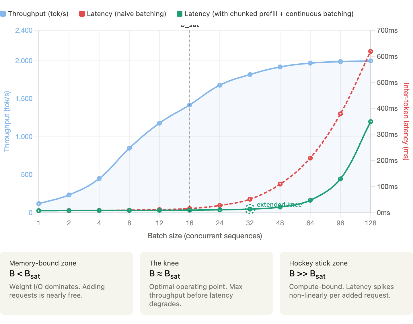
The chart above (created to illustrate hypothetically how throughput and latency typically behave as batch size grows) shows that below the saturation batch size (B_sat), you can get near-free throughput gains because GPU memory I/O is the bottleneck, and adding requests incurs almost no latency cost. Whereas in past B_sat, the system flips to compute-bound and latency hockey-sticks while optimizations like chunked prefill and continuous batching push that inflection point further right, giving you more headroom before the spike hits.
When to Optimize for Throughput vs. Latency
This is the decision that ultimately determines the cost structure, and there is no universal answer. It depends on workload, your users, and business model.
Before we see each workload type, let’s look at two fundamental principles that determine LLM performance:
- Little’s Law: Connecting QPS, Latency, and Concurrency
NoneConcurrency = QPS × Average Latency
If the system handles 10 QPS with an average end-to-end latency of two seconds, you have ~20 concurrent requests in flight. This tells you how many “slots” your system needs, which directly translates to batch size requirements, memory pressure (for 20 concurrent sequences), and GPU utilization.
Working backwards if your GPU can handle a maximum batch size of 32 and your target average latency is two seconds, your maximum QPS is 16. If you need 100 QPS, you need at least seven replicas, and at that point, the cost model becomes straightforward.
- The Roofline Model
The Roofline Model identifies whether your performance is capped by raw processing power (compute-bound) or by the speed at which data moves (memory-bound). Understanding this distinction is the key to not overpaying for hardware.
Here is how this model maps to the two phases of LLM inference:
| Phase | Bottleneck | Efficiency Target |
|---|---|---|
| Prfill (Input) | Compute | Processing lag prompt chunks in parallel |
| Decode (Output) | Memory | Loading model weights fo evry single token generated |
Latency-Sensitive Workloads
Some of the use cases where latency matters include interactive chat, code completion, real-time agents, search augmentation, and any user-facing application.
The primary SLO metrics that matter the most are TTFT (Time-To-First-Token) and ITL (Inter-Token-Latency). Users perceive TTFT as “responsiveness” and ITL as “streaming speed”.
How to tune
Keep batch sizes moderate since queuing would delay TTFT.
- Limit batch size to stay well below the B_Sat 'knee.
- In latency-critical apps, you are optimizing for P99 tail latency, not average throughput.
- Every request added to the batch increases the likelihood of a ‘prefill spike’ that delays everyone else’s tokens.
Use TP to minimize per-token latency (all GPUs working on every token).
- Scale Tensor Parallelism (TP) only within a single NVLink-connected node
- Once you cross nodes (using Ethernet or InfiniBand), the communication overhead between GPUs can actually increase ITL
- For latency-sensitive tasks, keep the model on the smallest number of GPUs that provide the necessary memory bandwidth.
Enable chunked prefill to prevent long prompts from blocking decode steps.
- Without chunking, a single massive prompt (e.g., a 20k token document) can “hijack” the GPU, forcing all other users to wait until the entire prefill is finished
- Breaking prompts into smaller chunks (e.g., 512 tokens) allows the engine to interleave prefill work with the decode steps of other active requests.
- This helps ensure that inter-token latency (ITL) remains consistent and allows the scheduler to fill “holes” in GPU compute cycles that would otherwise be wasted, balancing the high arithmetic intensity of prefill with the memory-bound nature of decode
Consider speculative decoding to reduce effective ITL.
- Speculative decoding trades compute efficiency for lower ITL by using a draft model to “guess” tokens ahead of time.
- This trades compute efficiency (OpEx cost) for lower ITL (Latency).
Over-provision slightly to handle traffic bursts without queuing.
- Higher cost per token (lower utilization with more GPUs for headroom), but necessary to meet user experience requirements.
Throughput-Sensitive Workloads
Some of the use cases where throughput trumps latency include batch summarization, offline data extraction, synthetic data generation, evaluation pipelines, and workloads where total job completion time matters more than individual request latency.
Tokens per second (or tokens per dollar) is the primary metric, and individual request latency is secondary as long as the total batch completes within the time window.
How to tune
Maximize batch size - push towards B_sat and beyond, accepting higher per-request latency.
- In the decode phase, the bottleneck is loading weights from memory.
- By increasing the batch size, you perform more arithmetic operations for every byte of weight data loaded.
- Push your batch size into the compute-bound territory (beyond the “knee” of the curve).
- While this increases the time for an individual token to generate, it can significantly increase the total Tokens Per Second (TPS) across the entire batch.
Use DP to add replicas and increase total throughput linearly.
- Unlike Tensor Parallelism (which splits a single request across GPUs to reduce latency), Data Parallelism runs independent model replicas on each GPU
- Use DP to scale throughput linearly. If one GPU handles 1,000 tokens/sec, four GPUs in a DP configuration will handle 4,000 tokens/sec.
- This helps avoid the “inter-GPU communication tax” that comes with trying to force low-latency parallelism on batch jobs
Increase the limit for concurrent token processing during the prefill phase to handle large prompt chunks more efficiently and maximize GPU utilization.
- Prefill is the most compute-intensive part of the process. To maximize throughput, you want to keep the GPU’s Tensor Cores fully occupied
- By processing massive chunks of tokens simultaneously, you ensure the GPU isn’t waiting for work, effectively “filling the pipe” and maximizing the FLOPS utilized per second.
Use aggressive quantization (INT4/GPTQ) if quality requirements permit. Throughput gain from fitting more in memory often exceeds the accuracy cost.
- Throughput is a function of how many sequences you can fit in VRAM
- Use 4-bit quantization to shrink the model weights and the KV Cache
- Even if individual token generation is slightly slower, the ability to process 4x as many concurrent sequences leads to a massive net gain in “Tokens per Dollar”
- While applying quantization, make sure the model is evaluated and accuracy hit is reasonable
Minimize over-provisioning - Run GPUs at high utilization since queuing is acceptable.
- In batch workloads, queuing is an asset, not a failure**.**
- A queue ensures that the moment one request finishes, another is ready to take its place
- Since there is no “Human-in-the-Loop” waiting for a response, you can ignore the “latency spike” that occurs at high utilization.
- Your metric for success is the total time to complete the entire job, which is minimized when the GPU never sits idle.
The Hybrid Reality
Most production systems aren’t purely one or the other. A typical deployment might serve interactive chat traffic during business hours (latency-sensitive) and run batch evaluation jobs overnight (throughput-sensitive).
Hence the cost-optimal approach is workload-aware scheduling:
- Dynamic autoscaling: Scale up GPU replicas during peak interactive hours, scale down during off-peak. The autoscaler should respond to both queue depth (reactive) and traffic forecasts (predictive).
- Priority queuing: Serve interactive requests at lower latency while processing batch requests in the background whenever spare capacity exists.
- Workload-specific configurations: Run different vLLM instances with different tuning parameters - one optimized for low-latency interactive traffic & another for high-throughput batch processing.
A Decision Framework
Given all of these trade-offs, how do you actually make a decision?
Here’s a decision framework to help:
Step 1: Characterize your workload
These include ISL/OSL distribution, QPS requirements (average and peak), and latency SLOs (TTFT and ITL at p50, p95, p99).
Step 2: Select your model and quantization
Start with the smallest model that meets your quality requirements. Benchmark FP8 first since it’s almost always worth the negligible accuracy trade-off. Only go to BF16 if you have a demonstrated quality regression in FP8.
Step 3: Benchmark on candidate hardware
Run your ISL/OSL sweep at varying QPS on at least two hardware options. Always trust measured throughput under your workload.
Step 4: Find the knee
For each hardware option, identify the maximum QPS that stays within your latency SLOs. This is your sustainable capacity per instance.
Step 5: Size your deployment
Use Little’s Law and peak QPS requirement to determine the number of instances needed. Add headroom for bursts (typically 20–30% above the knee).
Step 6: Calculate total cost
TCO_per_token = (Capital + Operational + Engineering Cost) / Total Lifetime Throughput
Compare the numbers across hardware options. Keep in mind that the cheapest GPU isn’t always the cheapest deployment.
Step 7: Plan for autoscaling
For variable traffic design autoscaling policies that trade cold-start latency for cost savings during off-peak hours. Fill spare capacity with batch workloads.
Build for Your Workload, Not the Benchmark
The throughput-latency-cost trilemma isn’t a problem to solve but a tension to manage. Every configuration choice you make shifts the balance between the three and there is no universally “perfect” configuration.
Teams that win in production don’t optimize based on spec sheets. They rely on rigorous benchmarking and workload characterization that provides a measured reality of specific prompts, models, and hardware.
While the serving frameworks and hardware landscape continue to mature quickly, the fundamental physics of LLM inference remain the same. While the tools for navigating this space are better than ever, the trilemma remains. To master it, stop guessing, start benchmarking, and tune your system to the metrics that actually matter to your business.
References
- HPCwire (NVIDIA DGX H100 launch specs): https://www.hpcwire.com/2022/03/22/nvidia-launches-hopper-h100-gpu-new-dgxs-and-grace-megachips/
- NVIDIA DGX H100 User Guide (official): https://docs.nvidia.com/dgx/dgxh100-user-guide/introduction-to-dgxh100.html
- Sunbird DCIM (cites 10.2 kW max): https://www.sunbirddcim.com/blog/can-your-racks-support-nvidia-dgx-h100-systems
- IntuitionLabs HGX guide (cites 10–11 kW): https://intuitionlabs.ai/articles/nvidia-hgx-data-center-requirements
- Syaala (GPU rack density analysis): https://syaala.com/blog/engineering-40kw-gpu-racks
- Introl (high-density rack guide): https://introl.com/blog/high-density-racks-100kw-ai-data-center-ocp-2025
- Silicon Data (H100 rental price history 2023–2025): https://www.silicondata.com/blog/h100-rental-price-over-time
- Introl (GPU cloud price collapse analysis): https://introl.com/blog/gpu-cloud-price-collapse-h100-market-december-2025
- GPUCloudList (2026 price guide with timeline): https://www.gpucloudlist.com/en/blog/nvidia-h100-price-guide-2026
- IntuitionLabs (rental price comparison): https://intuitionlabs.ai/articles/h100-rental-prices-cloud-comparison
- https://www.eia.gov/electricity/monthly/update/end-use.php (monthly update with sector breakdowns)
- DeepSeek-V3 technical paper: https://arxiv.org/abs/2412.19437
- Qwen3-235B-A22B-FP8 model card: https://huggingface.co/Qwen/Qwen3-235B-A22B-FP8
- FP8 Inference TCO paper: https://arxiv.org/abs/2502.01070
- NVIDIA Blackwell whitepaper: https://www.nvidia.com/en-us/data-center/technologies/blackwell-architecture/
- AMD MI350X announcement (Computex 2024): https://www.amd.com/en/products/accelerators/instinct/mi300x.html**
About the author
Related Articles

Mastering the 600B+ Frontier: Optimizing Large Model Deployments on the Inference Cloud
- April 21, 2026
- 9 min read
The Inference Cloud Memory Layer: A Technical Dive into DigitalOcean Managed Databases
- April 17, 2026
- 10 min read
Load Balancing and Scaling LLM Serving
- April 15, 2026
- 7 min read